In the process of doing business, an entrepreneur is faced with the need to finance his enterprise. He incurs fixed and variable costs to support his business activities. These costs are necessary to continuously produce products, provide services, or sell goods. Costs include various types: rental payments, staff salaries, costs of purchasing raw materials, materials or goods for sale, utility bills, payment for third-party services, and many others. Such costs have different economic meanings. Some of these costs are not directly related to the production of products, provision of services or sale of goods, while others, on the contrary, depend on this. Therefore, in the modern world it is customary to divide costs into fixed and variable costs .
Understanding fixed and variable costs is very important for an entrepreneur, as this allows you to competently manage your business .
The concept of variable and fixed costs
In this article, the concepts of fixed and variable costs, expenses and costs will be used interchangeably, although some scholars do not share these terms.
Variable costs are those company expenses that decrease or increase with production volume. In other words, the more products a company produces, the higher its variable costs and vice versa. Examples of variable expenses include piecework wages for workers, materials for production, electricity for production equipment, and payment for transporting goods.
Fixed costs are those expenses that a firm must always pay, no matter how much output it produces. There are fixed costs even when products are not produced at all. These include management salaries, electricity for office premises, depreciation, rent, etc.
Which costs are variable?
Variable costs are those that depend on the volume of production. That is, they increase when the scale of output increases and decrease when it decreases. The main feature that allows expenses to be classified as variable is their complete zeroing when production slows down.
Take our proprietary course on choosing stocks on the stock market → training course
Variable costs are the object of careful study in management accounting. Together with fixed costs, they constitute total costs, reserves for reducing which are usually sought precisely among their variable component.
The nature of the dependence of variable costs on production volume may be different. In accordance with this feature, such costs are divided into types presented in the table.
| Naming of expenditures | Description | Example |
| Proportional | An increase in production volumes entails an increase in the variable component of total expenses in the same proportion | Production volume increased by 25% and variable costs also increased by the same 25% |
| Degressive | Production volumes are growing at a much faster rate than variable costs | Production volume increased by 45%, and the variable component of all expenses by only 10% |
| Progressive | The growth rate of variable costs outpaces the rate of increase in output volumes | Production volume increased by only 20%, and variable costs increased by as much as 40% |
Also, variable costs are divided on the basis of attribution to cost into direct (which can be attributed directly to the manufacture of a specific type of product) and indirect (which also depend on production volumes, but they are very difficult to attribute to a specific type of product).
According to the method of inclusion in the production process, variable costs are divided into production and non-production.
Types of costs
In business it is very difficult to find “pure” variable and fixed expenses. This division is used to simplify the analysis. The types of variable and fixed costs in real life are semi-fixed and semi-variable costs.
Their peculiarity is that some of the costs are variable, and some are constant. An example is a worker’s wages, which consists of a salary and a bonus for each part made. The salary portion will be a fixed cost, and the additional payment for parts will be a variable cost.
conclusions
Concluding the article, we summarize the above. I think it has become clear that determining the value of the constants
gatherings is an extremely important and responsible matter. The success and efficiency of subsequent economic analysis depends on competent planning of the project’s expenditures.
In order to correctly draw up a business plan for your project, we recommend that you seek the services of developing this document from specialists in this field. You can also do it yourself, which will be more difficult. But to make the process easier, we recommend a ready-made business plan for an enterprise with a similar type of activity, and use the structure of this sample to build a concept for the development of your own project.
Graphical representation of variable and fixed costs
Variable costs appear as a straight line on a graph. The starting point is the origin because at zero production variable costs are zero. A graph is considered to be a linear function of the form:
- Y = k*x, where y is the value of variable costs in monetary terms, x is the quantity of products produced, k is the amount of variable costs per unit of production
The fixed cost graph is also straight, but not from the origin, but parallel to the horizontal axis. This is due to the already described features of fixed costs. The equation looks like:
- Y=k, where y, k is the value of fixed costs in monetary terms.
Formula
Average fixed (fixed) costs (AFC) are numerically equal to the result of dividing total fixed costs (FC) by output (Q):
AFC = FC/Q
The total costs (TC) of a firm are either fixed (FC) or variable (VC). This can be written mathematically as follows:
TC = FC + VC
If we divide both sides of the equation by output Q, we get:
TC/Q = FC/Q + VC/Q
ATC = AFC + AVC
The resulting equality shows that average fixed costs (costs) can also be defined as the difference between average total and average variable costs:
AFC = ATC - AVC
Analysis time interval
As the company develops and turnover increases, for example, when acquiring additional capacity or hiring new managers, fixed costs change. On the graph it looks like steps.
The division into variable and fixed costs can only be made in the short term. The fact is that in the long term, turnover grows, payments, rental prices and utility bills increase under the influence of inflation and other external factors. As a result, all company expenses become variable.
Interest on loans and wages in the form of bonuses are semi-fixed costs?
Yes, most often this is true. Conditionally fixed costs, like traditional fixed costs , do not correlate with the volume of goods produced, but in one way or another change over time due to other factors.
With regard to interest on loans, this is due to the fact that the share of the corresponding interest in the structure of monthly payments specified in the agreement with the bank in the first months of settlement is, as a rule, noticeably higher than in the last.
In turn, staff salaries, calculated primarily based on the size of the bonus component, are also likely to be very volatile. Such remuneration schemes are typical, for example, for sales managers and top managers.
Conditionally fixed costs, of course, also influence the determination of the break-even point of an enterprise, as well as any other costs.
CVP analysis
The “Cost – Volume – Profit” analysis is used to determine the volume of production at which a change from loss to profit occurs. This type of analysis can be represented graphically:
The “Total costs” line is formed by adding two straight lines: “Fixed costs” and “Variable costs”. The point where revenue and total costs intersect is called the break-even point. It reflects the situation when the profit is 0. To the left and right of the break-even point are areas of loss and profit.
CVP analysis is a simplified model for assessing the situation in a company. Like all other models, it has a number of limitations:
- The selling price per unit does not change.
- Variable costs per unit are constant.
- Total fixed costs are fixed.
- Everything the company produces is sold, without reserve.
- Changes in production volume are the only factor that affects fixed and variable costs in the cost of production.
- If a company sells more than one product, their revenue ratio does not change.
What costs depend on production volume
As noted above, the costs of an enterprise, based on the principle of dependence on production volume, are divided into constant and variable. This is necessary to optimize and plan all expenses, as well as to facilitate the search for ways to reduce them.
Individual expenses increase with production growth, that is, they depend on its volume. They are called variables. The most obvious feature of the variable components of all expenses is manifested in proportional expenses, which grow in the same proportions as the size of output.
Example. To create the product you need 6 liters of material. The cost of this material is 150 rubles per liter. It turns out that when producing 100 units of a product, the costs will be the following amount:
100*150*6 = 90,000 rubles.
Let's assume that the production volume doubles, that is, the output will no longer be 100, but 200 units of product. Then the cost will change as follows:
200*150*6 = 180,000 rubles.
That is, there is a direct proportional relationship here. A twofold increase in output entailed a twofold increase in expenses.
In the example considered, the so-called “economy of scale” was not taken into account. Many suppliers provide volume discounts, which makes costs less proportional to production volumes.
Examples of fixed costs
In almost any organization, the structure of fixed costs contains the following items:
- Depreciation charges for fixed assets (if the accounting policy adopts the linear method, which provides for uniform transfer of value);
- Remuneration for permanent salaried employees;
- Mandatory contributions to the payroll funds of these employees;
- Financing the recruitment and training (retraining) of staff;
- Management costs and administration costs;
- Representation expenses;
- Payment to landlords for the use of warehouses, workshops, etc.;
- Payment for housing and communal services;
- Financing of socially oriented objects on the balance sheet of the organization;
- Payment of interest rates;
- Payment of property taxes;
- Transfer of land tax;
- Payment for services provided by third-party companies (security, cargo transportation, advertising agencies, etc.).
In relation to the cost of production, such costs are usually indirect. That is, between specific types of products they are distributed in proportion to some base.
Break-even point and margin of financial strength
These figures can be calculated using a formula if you divide the costs into variable and fixed for your business. The formula for calculating the break-even point is as follows:
- Break-even point (in units) = Fixed costs / (product price - variable costs per unit)
If you multiply the break-even point in units by the price of the product, you get the amount of revenue for break-even production.
The formula works for enterprises producing only one type of product.
To calculate the margin of financial safety (FSA), you need to subtract the break-even point from the company’s revenue:
- ZFP = Revenue - Break-even point (in monetary terms)
The name of the indicator speaks for itself. It demonstrates the amount that a company can count on in case of unforeseen circumstances. The greater the margin of financial strength, the further the company is from an unprofitable state.
Results
Fixed costs have 2 key features: a relatively stable value, as well as a lack of correlation with the volume of output of goods or services. In turn, if only the 2nd criterion is met, then the corresponding costs are more appropriately classified as semi-fixed costs.
fixed costs most in demand when calculating the break-even point, as well as solving problems of optimizing a company’s business model through reasonable reduction of certain types of relevant costs.
You can learn more about other components of analyzing the economic efficiency of an enterprise in the articles:
- “Financial leverage ratio - formula for calculation”
- “Calculation of marginal profit (formula and nuances)”
You can find more complete information on the topic in ConsultantPlus. Free trial access to the system for 2 days.
Break-even point for multiple products
In reality, you rarely see a company producing one type of product. Therefore, a method was invented to calculate the break-even level for a set of products. However, it has one important limitation: the share of different products in the company's revenue must be constant. In other words, whenever X units of product A are sold, Y units of product B and Z units of product C are also sold.
To better understand how to calculate the indicator, consider an example.
A certain company produces and sells two products: lemonade and water. Water sells for $7 per unit and has variable costs of $2.94 per unit, while lemonade sells for $15 per unit and has variable costs of $4.50 per unit. The marketing department estimates that for every 5 units of water sold, 1 unit of lemonade will be sold. The organization's fixed production and management costs are $36,000.
Let's calculate the break-even point for this company.
Step one: calculate the difference between price and variable costs per unit of production. This difference is also called the specific contribution margin.
- For water: 7 - 2.94 = $4.06
- For lemonade: 15 – 4.5 = 10.5 dollars.
Step two: calculate the marginal profit for the product set.
- (4.06 * 5) + (10.5 * 1) = $30.8
Step three: substitute the values into the break-even point formula:
- 36,000 / 30.8 = 1169 sets
Step four: calculate the number of products of each item that must be sold to make zero profit.
- 1169 * 5 = 5,845 bottles of water
- 1169 * 1 = 1169 bottles of lemonade
Step five: calculate the break-even point in monetary terms.
- (5845 * 7) + (1169 * 15) = $58,450
In order for production not to be unprofitable, the company needs to receive revenue of $58,450. Let us recall that this figure is correct only if five bottles of water are sold for every bottle of lemonade.
Marginal profit and direct costing system
In the Direct Costing system, the cost of each type of product (service) is determined in terms of only variable costs. Fixed costs in total are included in the financial result.
This system is used for management accounting purposes. After all, it has a great advantage. The direct costing system, due to the fact that fixed costs are not distributed among types of products, shows which type of product is more profitable for the enterprise. The analysis is carried out on the basis of marginal profit analysis.
For comparison, in a general costing system, the constant part is divided proportionally to the selected basis for calculations. This could be, for example, output volume, direct costs, workers' wages, etc.
where M1 is the marginal profit per unit of production (margin per unit of production), p is the price; AVC - average variable costs;
where M is gross marginal profit (gross margin); TR is gross revenue and VC is total variable cost.
Margin analysis
This type of analysis is used to select the most profitable products. To apply it, it is necessary to divide costs into variable and fixed. The basic premise is that the capacity of any business is limited. The main concept is marginal income (MI) or marginal profit. The formula for calculating marginal income is:
- MD = Revenue - Variable costs
Or:
- MD = Profit + Fixed costs
Since fixed costs are shared across the entire enterprise, high-margin products should be prioritized. For clarity, let's look at an example again.
The company produces 3 types of products: crackers, chips and corn sticks. Prices, variable costs per unit and specific contribution margin are presented in the table:
| Product | price, rub. | Specific variable costs, rub. | Specific MD, rub. |
| Crackers | 15 | 5 | 10 |
| Chips | 40 | 20 | 20 |
| Corn sticks | 30 | 8 | 22 |
The company can only produce 20,000 packages per month. The maximum quantity of each type of product that can be produced: crackers - 14,000 packages, chips - 10,000, corn sticks - 8,000.
The maximum MD will be:
- (22 * 8000) + (20 * 10,000) + (10 * 2000) = 396,000 rub.
You can independently calculate the marginal income for all combinations and make sure that a set of 8,000 packs of corn sticks, 10,000 packs of chips and 2,000 packs of crackers is the most profitable.
Using marginal analysis, we used all production capacities and selected the most profitable set of products.
Examples of calculating the break-even point
Example 1: Calculation of critical volume
The current sales volume of the travel agency was 145 tours with an average bill of 25,000 rubles;
variable costs per unit of production – 14,200 rubles; total fixed costs for the year – 1,024,000 thousand rubles. It is necessary to determine at what volume of production the enterprise operates without profit or loss. vouchers _
Consequently, the company will make a profit when selling more than 95 vouchers. Or in other words, the critical sales volume is 95 vouchers.
Example 2. Break-even point and margin of safety
Based on example 1, find the safety margin of the investment project in value and physical terms.
Safety margin of vouchers.
Safety margin of rubles.
Example 3. Building a break-even chart
Let's look at a graphical representation of the break-even point based on the previous example.
Break-even point chart
Thus, the model for determining the break-even point (critical volume, break-even threshold, profitability threshold) allows you to solve several problems. First, find the volume at which the enterprise or project does not make a profit, but also does not incur losses. Secondly, find the safety margin of the project. Third, assess potential risks.
The model for calculating the break-even point (critical production volume) is the simplest way to analyze project risks.
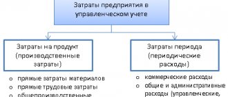
Fixed and variable expenses in accounting
Accounting for fixed and variable costs is optional. It is used by managers to make management decisions. However, in accounting, this division can be useful when calculating costs using the “Direct Costing” method.
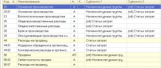
It also adds a division into direct and indirect costs. The essence of this method of cost accounting is that the costs of producing products form production costs, and general business costs are written off as period expenses. The cost of production is accumulated on account 25, and production maintenance costs are accumulated on account 26. The entire amount of the 26th account is written off as expenses for the period, regardless of how many products were sold.
What is the break-even point?
The break-even point is also called the critical production volume, break-even threshold or profitability threshold.
even point (critical point, CVP-point) is the volume of sales at which the company does not incur losses, but does not make a profit.
The break-even model is based on the Direct Costing cost determination system. In this system, the truncated cost is calculated, as well as the marginal profit (margin) is determined.
To determine the critical volume (break-even point), it is necessary to plot gross revenue ( TR - Total Result) and total costs ( TC - Total Cost) on one graph.
Calculation of variable production costs
How to calculate variable costs? Very simple. To find their total amount for the period, you need to add up all the costs that are defined as variables.
It is convenient to use accounting data from the accounting accounts discussed above for this purpose. It should be taken into account that in accounting there is no division into fixed and variable costs, but the existing direct costing method allows them to be divided in this way, according to which fixed costs can be written off as a decrease in the financial result at a time.
In the cost sharing situations we discussed above in small and large organizations, it will look like this:
- Small enterprises that use only two accounts (20 and 26) to collect costs will take into account as variables the amount of costs that during the period under review will be written off from account 20 (if the company provides services) to the debit of account 90 or from account 20 to the debit of account 43 (if we are talking about finished products). In the first case, for the period corresponding to the reporting period, this amount can be taken from line 2120 of the financial results report. In the second, variable costs will fall into the same line of Form 2 if the volumes of products produced and sold during the period coincide.
For information on the procedure for entering data into the lines of the financial results report, read the article “Filling out Form 2 of the balance sheet (sample)”
- Trade organizations that use only one account 44 to account for costs will highlight among them those that are defined as variable (costs of packaging goods, interest and rewards paid for sales, with charges on them), and, adding their sum with the cost of goods sold (which will be equal to the volume of debit from account 41 to the debit of account 90), they will receive the total amount of variable costs for the period under review. It will not be possible to take this data directly from the accounting records.
- Large organizations that use all existing accounts (20, 23, 25, 26, 44) to account for costs and have decided to classify expenses collected on account 25 as variable, variable costs for the period will be determined as the cost of finished products written off from account 20 to the debit of account 43, or as the cost of services written off from account 20 to the debit of account 90. If the organization does not carry out trading activities and does not need to divide the costs collected on account 44, then for the reporting period the volume of variable costs for services can also be taken from line 2120 of the financial results report. Data on finished products will fall into this line if the volumes of produced and sold products coincide for the period under review.
PI = ∑ З,
where: PI - variable costs;
Z - costs incurred in connection with the direct creation of sold goods (works, services) and taken into account in their cost. They must be summed up, but the expenses included in the cost price when distributing account 26 must be excluded from them.
Categories
The problem of distribution of fixed costs in production
At any stage of a company's life, there are always challenges to accounting and cost management. To determine how much needs to be sold and at what price for a given product to bring profit to the company, it is necessary to calculate how much it costs to produce a particular type of product.
The fact that all costs must be divided by type of product is an indisputable issue. The only catch is the principle by which costs should be divided. After all, the costs of an enterprise in the process of production and marketing of goods and services are taken into account in different ways. Conventionally, they can be divided into fixed and variable costs. Variable costs directly depend on the volume of production at the enterprise. The basis of variable expenses is the use of working capital (working capital). These are raw materials, materials, fuel, electricity, direct labor of workers, as well as services of third-party organizations related to the production of specific products, etc. Fixed costs are associated with compensation for related production factors. Their sizes do not directly depend on the volume of products produced. Fixed expenses include rent for production premises and warehouses, depreciation of capital equipment, security, general business expenses associated with the maintenance of employees of the administrative apparatus, accounting department and warehouse, etc.
If production stops in any month, variable costs will drop to almost zero. At the same time, fixed costs will remain at approximately the same level: it will still be necessary to pay the salaries of some of the administrative employees conditionally assigned to this production, pay rent for this premises, pay security, and also charge depreciation of equipment.
By comparing variable and fixed production costs at a particular enterprise, managers can influence the economic policy of the company, because the cost of goods sold is, in essence, the total sum of all the costs of the enterprise. At the same time, variable costs are almost always subject to accurate accounting at the enterprise, but there are known difficulties with regard to the distribution of fixed costs by type of product. Therefore, in practice, when taking into account fixed costs, the question often arises: is it worth distributing fixed overhead costs across types of products or can this be done without? Accordingly, there are two approaches. In the first approach, these costs are established per product group or per production unit - this is the so-called mixed (combined) approach to the analysis of fixed costs. The second approach requires localization of fixed overhead costs by product type.
Depending on the approach used or the method of accounting for fixed costs, sometimes even directly opposite results can be obtained. This article compares these methods and evaluates both the positive and negative aspects of their use.
Combined fixed cost analysis
Some experts quite reasonably believe that the use of this method is appropriate when assessing the efficiency of production of products for the entire enterprise. In practice, especially with a small range of production and sales and a simple structure of overhead costs, they usually do not resort to separate accounting of fixed costs . The main assumptions when considering this method are as follows:
- variable costs are localized by product;
- fixed costs are considered as a total for the enterprise as a whole;
- marginal profit is estimated for each product;
- profitability, as well as other financial indicators (for example, safety margins) are assessed for the entire enterprise as a whole.
This approach has obvious advantages: ease of calculation and no need to collect a large amount of data. The disadvantage of this approach is the impossibility of comparative assessment of profitability for individual types of products.
Example 1
The manufacturing company produces chemicals for automobile use. The production range is presented in table. 1. For simplicity of calculations, we will limit ourselves to three product names.
Having orders for three products in their portfolio, the company's managers decided to analyze the profitability of each type of product. At first, they used the first approach, that is, they did not divide indirect costs by elements of the product portfolio. Having identified the main variable costs, they obtained the following results for a comparative analysis of product profitability (see Table 1; in the table, all calculations are shown in a monthly breakdown of the company’s activities).
Judging by the data in Table. 1, a feature of the order portfolio is its lack of balance. Indeed, glass cleaner ranks second in terms of profitability (in %) among all products. And at the same time, this type of product ranks last in terms of sales volume (revenue). As a result, the profitability of the sales portfolio as a whole (10%) leaves much to be desired. Therefore, to increase the efficiency of production and sales, company managers should focus their efforts on “promoting” this product.
Next, we will evaluate the company’s financial stability to changes in external economic conditions. In this sense, an important condition for the successful operation of an enterprise is the safety margin. The margin of safety, or financial strength, shows how much sales (production) of products can be reduced without incurring losses. The excess of real production over the profitability threshold is the margin of financial strength of the enterprise. This indicator is defined as the difference between the planned sales volume and the break-even point of the business (in relative terms). The higher this indicator, the safer the entrepreneur feels in the face of the threat of negative changes (for example, in the event of a drop in revenue or an increase in costs). The break-even point is usually presented in physical (units of production) or monetary terms. It can be stated with certainty that the lower the break-even point, the more efficiently the enterprise operates in terms of generating operating profit. Let's calculate the break-even point for the entire production and sales portfolio. The break-even point of a business is easy to find if the financial result from product sales is equal to zero. To do this, the marginal profit (MP) from sales is equated to fixed costs (Zpost):
MP = Zpost.
In this case, the company will have neither profit nor loss. Then the critical sales volume or critical revenue (Vkr), at which there is neither profit nor loss, can be found from the following ratio:
(MP / Vpr) × Vkr = Zdc.
The meaning of this formula is that when current sales revenue (Vpr) drops to its critical level (Vkr), their values will decrease. In this case, there will be no profit (MP = Zpost). Next, we write this formula in the following form:
MP / Vpr = Zpost / Vkr.
In this formula, the first part of the equality is an expression for determining the profitability of the enterprise’s products as a whole in terms of marginal profit. Let's denote it by the indicator:
^(MP) = MP / Vpr.
Further according to the table. 1 we find the value ^(MP): (1050 thousand rubles /2500 thousand rubles) × 100% = 42.0%.
Hence, the critical revenue (or break-even point) (Vkr) in monetary terms is equal to: 800 thousand rubles. / 0.42 = 1905 thousand rubles.
The safety margin factor (Kzb) will be: [(2500 – 1905) / 2500] × 100% = (595 / 2500) × 100% = 23.8%.
In its meaning, KZB characterizes the break-even point in monetary terms. This is the minimum income at which all costs are fully recouped, while the profit is zero. It is believed that for normal operation of an enterprise it is quite enough if the current sales volume (Vpr) exceeds its critical level (Vkr) by at least 20%. In this case, this figure exceeds the recommended value, but is almost on the verge.
It would seem that everything is clear: on the one hand, in the general case we have an unbalanced structure of production and sales of the order portfolio for total products, on the other hand, there are relatively low profitability indicators and safety margins for the company’s products as a whole. In addition, it appears that we have rather meager information about the behavior of fixed costs in relation to each type of product. However, the presented picture may change radically if we take into account the distribution of fixed costs by type of product.
| Table 1. Impact of product structure on profitability and break-even point | |||||||||
| Index | Revenue, thousand rubles | Variable costs, thousand rubles. | Marginal profit, thousand rubles. | Marginal profit, % | Fixed costs, thousand rubles. | Break-even point thousand rubles | Safety margin, % | Operating profit, thousand rub. | Profitability, % |
| Brake fluid | 1350 | 750 | 600 | 44,4 | |||||
| Glass cleaner | 500 | 300 | 200 | 40,0 | |||||
| Solvent for laminar film removal | 650 | 400 | 250 | 38,5 | |||||
| Total | 2500 | 1450 | 1050 | 42,0 | 800 | 1905 | 23,8 | 250 | 10,0 |
Baseline method
If the company's management requires more complete information to make management decisions, then you can use the basic indicators method . In this case, it is necessary to localize fixed costs by type of product. The main assumptions of this approach are as follows:
- variable costs are distributed across products;
- fixed costs are also localized by product;
- contribution margin is estimated for each product;
- Safety margin and profitability are assessed for each product.
Using the basic indicators method, the company has the opportunity to make a complete comparative assessment of the profitability of individual types of products - an undoubted advantage of this approach. In this case, an indicator is selected as the basis for the distribution of fixed costs, the value of which is closely related to the type of costs under consideration. Typically in the economic literature the following values are taken as such an indicator:
- the volume of work produced or sales for each type of product;
- production areas for each type of product;
- the complexity of manufacturing certain types of products;
- wages of production workers attributable to each type of product;
- other indicators.
The procedure for selecting a base indicator requires the fulfillment of at least two conditions:
1) preliminary analysis of the relationship between the localized type of costs and one of the selected basic indicators;
2) organization of accurate measurement and accounting of the influence of the base indicator on the localized type of overhead costs.
The better the indirect costs are attributed to a specific product as they appear in production, the more accurately its total cost of production can be calculated.
Example 2
We use the data from the previous example, but expand it somewhat - now there is much more information for analysis (Table 2).
Suppose the company's management decided to redistribute fixed costs to each type of product in proportion to the wages of production workers. To justify their decision, managers referred to the large share of labor costs in the cost of manufacturing each product. Taking into account the choice of this basic indicator, the calculation of the cost of the mentioned products is as follows (see Table 2).
| Table 2. Allocation of fixed costs using the base indicator | ||||
| No. | Index | Brake fluid | Means for washing glasses | Solvent for laminar film removal |
| 1 | Variable costs, rub. | 750 000 | 300 000 | 400 000 |
| 2 | Quantity of products, pcs. | 15 000 | 10 000 | 5000 |
| 3 | Variable costs per unit of production, rub./piece. (item 1 / item 2) | 50,0 | 30,0 | 80,0 |
| 4 | Salaries of production workers, % | 55 | 15 | 30 |
| 5 | Distribution of fixed costs, rub. | 440 000 | 120 000 | 240 000 |
| 6 | Fixed costs per unit of production, rub./piece. (clause 5 / clause 2) | 29,33 | 12,0 | 48,0 |
| 7 | Cost per unit of production, rub./pc. (item 3 + item 6) | 79,33 | 42,0 | 128,0 |
| 8 | Sales price, rub./pcs. | 90,0 | 50,0 | 130,0 |
| 9 | Revenue, rub. (p. 2 × p.  | 1 350 000 | 500 000 | 650 000 |
| 10 | Product profitability, % | 11,9 | 16,0 | 1,6 |
| 11 | Break-even point, rub. | 990 000 | 300 000 | 624 000 |
| 12 | Safety margin, % | 26,7 | 40,0 | 4,0 |
In table 2 data in natural units (pieces) is the number of bottles or canisters filled with the corresponding liquid for car maintenance. As you can see, glass washer is the leader in profitability. With the current distribution of fixed costs (proportional to salary), the profitability value for it is 10 times higher than the same indicator for solvent for removing laminar film (16% / 1.6%) and more than 1.3 times higher compared to the same indicator for brake film. liquids (16% / 11.9%). The value of product profitability (^(Ppr)) was determined as the difference between sales prices (Tspr) and the total cost of a unit of production (Full) according to the formula:
^(Ppr) = (Cpr – Full) / Cpr × 100%.
The indicator ^(Ppr) is often also called the price coefficient . The higher the value of this coefficient, the higher the potential profitability of a given product, which means the greater the reserve for covering overhead costs and making a profit. In other words, it is most profitable to sell products with the highest price coefficient.
To calculate the break-even point of a business by type of product, we will use a different approach - we will use a simple ratio based on the balance of revenue and costs of the enterprise. Let's do this consistently for all types of products. For brake fluid in the absence of profit, we obtain the following equation:
90X = 50X + 440,000 + 0.
In this equation, X is the required number of units of production (brake fluid). At this unit value there is no profit or loss. Zero in this formula means no profit. Having solved this equation, we obtain the required number of units of production:
X = 440,000 / 40 = 11,000 pcs.
Hence the critical sales volume in value terms (revenue) will be:
11,000 pcs. × 90 rub./pcs. = 990,000 rub.
Now let's determine the safety margin:
[(1 350 000 – 990 000) / 1 350 000] × 100 % = (360 000 / 1 350 000) × 100 % = 26,7 %.
For glass washer, we find the break-even point from a similar equation:
50X = 30X + 120,000.
Hence the critical volume of production in natural units will be:
X = 120,000 / 20 = 6000 pcs.
Critical revenue will be:
6,000 pcs. x 50 RUR/pcs. = 300,000 rub.
Then the safety margin will be:
[(500 000 – 300 000) / 500 000] × 100 % = (200 000 / 500 000) × 100 % = 40,0 %.
Let's create a similar equation for the solvent for removing laminar film :
130X = 80X + 240,000.
Let us determine the critical volume of production in natural units:
X = 240,000 / 50 = 4800 pcs.
In turn, critical revenue will be equal to:
4800 pcs. × 130 RUR/pcs. = 624,000 rub.,
and the safety margin will be:
[(650 000 – 624 000) / 650 000] × 100 % = (26 000 / 650 000) × 100 % = 4,0 %.
It follows that in terms of the safety margin for the second product ( glass washer ), we got an excellent result: the current sales volume is 40% higher than its critical level (break-even point). The first product ( brake fluid ) also achieved good results, although its break-even point was 26.7% lower. The worst result of the safety margin is for the third product ( laminar film remover ): in this case, the break-even point differs from the current sales level by only 4%. This means that if sales volume drops by at least 200 pcs. (26,000 rubles / 130 rubles), there will be no profit on this product. And with a further drop in sales volumes there will be continuous losses. It turns out that from all points of view the worst results are produced by the release of the third product ( solvent for removing laminar film ). Given current sales volumes and prices, this product practically does not justify the costs of its production. To increase the efficiency of its production, it is necessary to increase production volumes or selling prices.
Or maybe everything is not so bad with the release of solvent for removing laminar film? After all, from the data in Table. 1 it follows that the marginal profit for it (38.5%) is not much worse than for the second product (40%). Probably, managers incorrectly chose the base indicator for the distribution of fixed costs: it was necessary to take into account not one, but two base indicators or more. That is, for different components of indirect costs it was necessary to choose their own basic indicators depending on the sources of the corresponding costs (see example 3).
ABC method
In economic terms, indirect costs should be attributed to one or another type of product in accordance with the extent to which these costs are related to the production of a particular product. In other words, in the process of allocating general production costs, it is necessary to clarify to what extent the cost elements are associated with the production of a particular type of product. During the analysis process, it may turn out that some indirect costs are directly related only to a specific product, so it is unfair to redistribute them to all products. In these cases, indirect costs are correctly attributed to the product according to the place or sources of their occurrence. To allocate such costs in a similar manner, a method called Activity Based Costing (ABC method) can be used. This phrase is translated from English in different ways: cost analysis by type of activity, operational cost analysis, and even functional cost analysis (FCA). Regardless of the translation into the basis of this method, the task is to find a different (not related to the volume of sales) basis for allocating overhead costs.
In connection with the above, let’s return to the company’s product portfolio (examples 1, 2).
Example 3
The manager is not confident in the results obtained regarding the comparative profitability of products, so he demanded to present a full line of indirect cost elements. Managers localized fixed indirect costs by type of product (the results are summarized in Table 3). It turned out that at first they did not take into account that for the production of the second product ( glass washer ) an automatic line was purchased on a long-term lease basis. To accommodate this equipment, it was necessary to rent additional premises, while other workshops are owned by the company. As a result, in the previous calculation, fixed costs were artificially redistributed to other products in proportion to wages. After all, an automated line requires less labor than other products. This will result in lower labor costs. Therefore, when distributing costs in proportion to the salaries of the main workers, the lion's share of the costs fell on the neighbors of this product, that is, on the first and third products, the production of which is not as automated. In reality, it was in connection with the production of the second product ( glass washer ) that the company incurred two significant cost elements - leasing and rental payments. Therefore, it is this product that must recoup these costs with income from its sales. And if so, then these costs should be fully allocated to the production of the second product.
Let's assume that in this case they total 150 thousand rubles. per month. To do this, they must first be separated from the total amount of fixed costs (800 thousand rubles): 800 – 150 = 650 rubles. But the remaining amount of costs (650 thousand rubles) can be distributed in proportion to the salaries of production workers. The results of the redistribution of fixed costs are presented in table. 3.
| Table 3. Allocation of fixed costs by place of their occurrence ( ABC method) | ||||
| No. | Index | Brake fluid | Means for washing glasses | Solvent for laminar film removal |
| 1 | Variable costs, rub. | 750 000 | 300 000 | 400 000 |
| 2 | Quantity of products, pcs. | 15 000 | 10 000 | 5000 |
| 3 | Variable costs per unit of production, rub./piece. (item 1 / item 2) | 50,0 | 30,0 | 80,0 |
| 4 | Salaries of production workers, % | 55 | 15 | 30 |
| 5 | Leasing payments and rental of additional production premises, rub. | — | 150 000 | — |
| 6 | Distribution of other fixed costs, rub. | 357 500 | 97 500 | 195 000 |
| 7 | Total fixed costs, rub. (item 5 + item 6) | 357 500 | 247 500 | 195 000 |
| 8 | Fixed costs per unit of production, rub./piece. (clause 7 / clause 2) | 23,83 | 24,75 | 39,0 |
| 9 | Cost per unit of production, rub./pc. (item 3 + item | 73,83 | 54,75 | 119,0 |
| 10 | Sales price, rub./pcs. | 90,0 | 50,0 | 130,0 |
| 11 | Revenue, rub. (item 2 × item 10) | 1 350 000 | 500 000 | 650 000 |
| 12 | Product profitability, % | 21,9 | –9,5 | 8,5 |
| 13 | Break-even point, rub. | 804 420 | 618 750 | 507 000 |
| 14 | Safety margin, % | 40,4 | –27,8 | 22,0 |
As we can see, the picture has changed a lot. Now the fixed costs per unit of production for the second product are the highest (24.75 rubles/piece). As a result, its total cost increased sharply, and the sale became unprofitable - at 4.75 rubles. for each piece of product. The leader in profitability was the first product - at 21.9%. The production of the third product can also be rehabilitated. Compared to the previous calculation, its profitability increased more than 5 times (8.5% / 1.6%). And why all? Yes, because the structure of fixed costs has changed. For clarity, let us present these results in graphical form (Fig. 1). This figure shows the distribution of fixed costs for Example 2 (baseline method); the designation of products 1, 2 and 3 corresponds to their sequence in the table. 2. Similarly, we show the distribution of fixed costs using the ABC method in Fig. 2.
Rice. 1. Diagram of distribution of fixed costs using the base indicator method
Rice. 2. Diagram of distribution of fixed costs the ABC method
As we can see, with the transition to a more objective evaluation method (ABC method), the share of fixed costs for the second product ( glass washer ) increased more than 2 times - from 15 to 30.94%. Accordingly, the share of costs for the first and third products decreased. This explains the significant deterioration in overall profitability for product 2.
Next, as in previous examples, we will calculate the break-even point and safety margin for all types of products, using the data presented in table. 3. For the first product ( brake fluid ), we create the following equation:
90X = 50X + 357,500.
From here we get the following number of units of production:
X = 357,500 / 40 = 8938 pcs.
The critical sales volume (revenue) will be:
8038 pcs. × 90 rub./pcs. = 804,420 rub.
Now let's determine the safety margin:
[(1 350 000 – 804 420) / 1 350 000] × 100 % = (545 580 / 1 350 000) × 100 % = 40,4 %.
For the second product ( glass washer ), we find the break-even point from a similar equation:
50X = 30X + 247,500,
from where we determine the critical volume of production in natural units:
X = 247,500 / 20 = 12,375 pcs.
Critical revenue will be:
12,375 pcs. × 50 RUR/pcs. = 618,750 rub.
The safety margin will be equal to:
[(500 000 – 618 750) / 500 000] × 100 % = (–118 750 / 500 000) × 100 % = –27,8 %.
For the third product ( solvent for removing laminar film ) we will also create a similar equation:
130X = 80X + 195,000.
Let us determine the critical volume of production in natural units:
X = 195,000 / 50 = 3900 pcs.
In turn, critical revenue will be:
3900 pcs. × 130 RUR/pcs. = 507,000 rub.,
where does the safety margin come from:
[(650 000 – 507 000) / 650 000.] × 100 % = (143 000 / 650 000) × 100 % = 22,0 %.
As one would expect, the first product has the largest safety margin (40.4%). This indicator is followed by the third product (22.0%). And for the second product, the current sales level is even below the breakeven point - by 27.8%. This explains the negative result for the safety margin of this product (–27.8%). Everything fell into place. The glass cleaner turned out to be the “weak link” in the company’s product portfolio. This product generates a loss and drags down the entire portfolio of the plant's commercial products.
However, the fact that this product is unprofitable at full cost does not negate its potential capabilities, because in terms of marginal profitability it is in second place. Unprofitability at full cost indicates that the current volumes and sales prices are not enough to cover the costs of its production. In this case, the company made an error in planning prices or volume of production and, as a result, did not receive the revenue required to fully cover its costs. If the sales volume is increased, then, in the end, it will be possible to overcome this negative impact of the costs of the second product. Then the second product may turn out to be even more profitable than the third.
Thus, example 3 shows that the use of the ABC method allows for a more reasonable allocation of fixed costs by type of product. You just need to correctly select for each product the determining factors that influence the composition of fixed costs. Summarizing what has been said, we can recommend the use of a system for localizing fixed costs according to basic indicators for such cases:
- simple and similar types of products or services;
- low level and simple structure of overhead costs;
- low sales and administrative costs;
- high sales profitability.
The use of the ABC method is advisable if the business is characterized by the following features:
- multi-item order portfolio;
- high share of indirect costs;
- significant differences in production volumes of certain types of products;
- Enterprise managers strive to deeply understand the cost structure.
Note that the ABC system, which is so actively supported in principle, at the same time has not yet found wide distribution, including in Western enterprises. The main reason is the complexity and unfamiliarity of the transition from the traditional system existing at enterprises (localization of costs according to basic indicators).
Conclusion
Generalization of experience allows us to argue that the basis for managing indirect costs should be the principle of reasonable necessity, which assumes that the potential benefits of a more detailed consideration and distribution of indirect costs should outweigh the efforts associated with such deepening. Based on this principle, we examined different methods for assessing efficiency for multi-item production.
The method of comparative evaluation of individual types of products based on marginal profit is very simple to use. However, it allows for an assessment of profitability only with a combined analysis of fixed indirect or indirect costs. The basic indicator method allows the enterprise to make a complete comparative assessment of the profitability of individual products among themselves, but does not allow either to trace overhead costs or to manage them in a reasonable manner. The use of the ABC method allows for a more reasonable allocation of fixed costs by type of product. Redistribution of cost elements between individual products allows you to significantly change your view of the real share of profit that a particular type of product brings. This is especially significant in the case of analyzing types of products that, due to the indirect costs associated with them, turn out to be unprofitable for the business. True, the complexity of using this method is greater than the simpler assessment methods listed above.